
I thought this must be what finishing a marathon feels like when I submitted this report, my first hands-on machine learning project. I was making mental plans to celebrate with my friends as I cheekily included a "have fun reading this long report :)" comment for my professor in the submission box, I think he took it well. Here's a major shoutout to my team members Rittika Mitra, Kabita Paul, Namrata Tathe, and Ibrokhim Sadikov, for the collective responsibility we carried as we scrambled to make deadlines, train our models, and improve results tirelessly. In this post, I'm excited to share the analytical methods we undertook to predict risk of credit default for Home Credit.
Home Credit is a financial institution that aims to create lines of credit specifically for the unbanked population. Unlike other credit institutions, the major challenge of Home Credit to predict loan default is absence of Credit score. The main target clients of Home Credit are unbanked or underbanked population with very limited credit history. The objective of this project is to build effective and efficient classification model to predict applicants’ loan repayment ability and to minimize risks of credit default for Home Credit.
Data Profile
We collected our data from Kaggle, an online community that allows data science practitioners access to public data and post their solutions. There are a total of seven tables provided with the problem. For full details on each table, please click on this link: Kaggle Home Credit.Before we tackle the problem, we have identified a few constraints in our preliminary assessment of the data:
1. Too many attributes
The application table alone contains 122 variables. If we include other supplementary tables in our model, we would have 400+ variables in total. We need to carefully choose variables that are important for our analysis in order to minimize noise without losing valuable information. In order to do this, we elected to use feature selection which will be further explained in the data preprocessing step.2. Dealing with Missing values
There are high percentage of missing values for few attributes. There are many ways to handle missing values. Most common methods are dropping records with missing values (when the percentage of missing value is low). One other method is to discard columns with high number of missing values. Missing values can be handled by Imputation techniques as well. In imputation, missing values for categorical variables are replaced by either most frequently used category or considered as a third category. During our initial stage, we preferred imputation over dropping in order to avoid loss of information.3. Imbalanced Data
The application dataset contains less than 10% records in which the target variable equals to 1. This means less than 10% of the clients have defaulted in the past. This is good news for the company, but when building model, we have to design it in a way so that the algorithim will not be biased towards the category with high number of observations (in this case, it's the paid application category, or target=0).Exploratory Data Analysis
Due to the high volume of data, we want to pinpoint information that’s most relevant to our model in order to achieve our objectives. We will start off by looking at current applicant information from the application tables. Together the application_train and application_test tables have a total of 356255 records, which means there are currently 356255 applicants in the system. An important point to note is that the application_test dataset does not contain a target variable. When we are ready to run our model, we need to split the application_train table into train and validation datasets.In order to better understand the risk of default, we want to use the TARGET variable from the application_train dataset and compare it to various predictors. Here, a value of 0 represents a repaid loan, while a value of 1 represents a default loan. Before we proceed with modelling, we want to first understand the distribution of the target variable, as shown below:
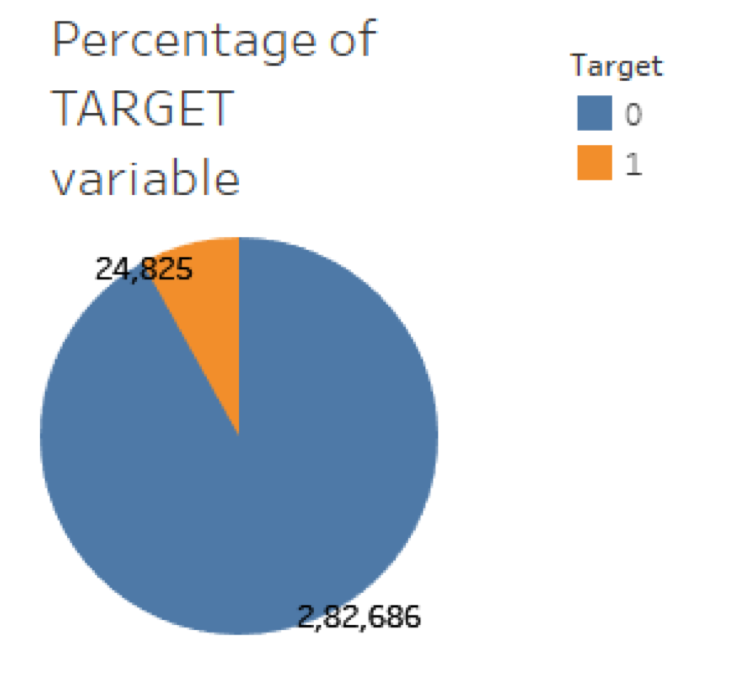
As we can see, class 0 is significantly larger than category 1. This means only a few loans were not repaid compared to loans that are repaid. When classes are imbalanced, machine learning models are biased towards category with higher number of observations. The classifier will achieve a high accuracy based on the majority class. This doesn’t make a good predictive model because the minority class will simply be ignored. Another important point to note is that the application_test dataset does not contain a target variable. When we are ready to run our model, we need to split the application_train dataset. We have shown data distribution of applicant’s general information below:
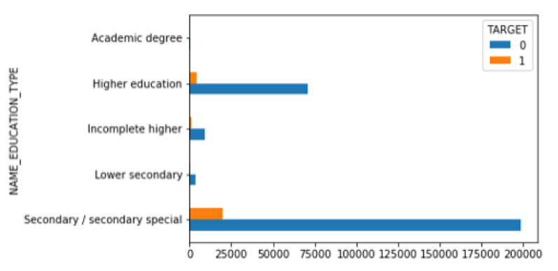
Applicant Education
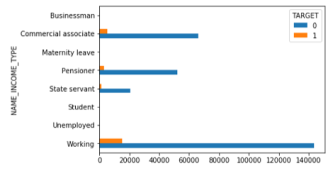
Applicant Income Type
Type of Loan
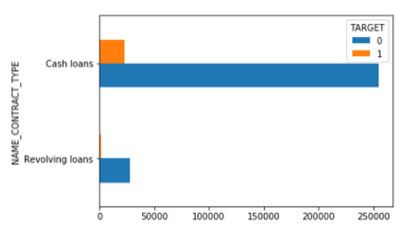
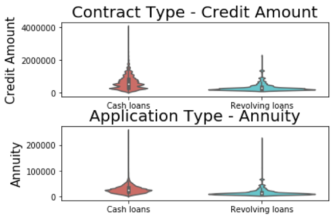
As we can see in the distribution graph above, most applicants prefer cash loans over revolving cash. To take a deeper look into applicants’ financial background, we wanted to visualize the differentiation in credit amount and annuity data between applicants applying for different types of loans.
Credit amount and annuity distributions per contract type:
We also observed that the previous application table contain large amount of information that may be useful to our analytics model. The previous application table contains a “SK_ID_PREV” (ID for previous applications) field and a “SK_ID_CURR” (ID for current applications) field. This could allow us to map previous application records back to current application. In addition, we noticed that many current application IDs are linked to more than one previous application IDs. This means most current applicants have previously applied for loans.
To get a better understanding, we counted the number of previous application records for each current applicant using the group_by statement on SK_ID_CURR. Here's an example of how you can do it using R:
    library(dplyr)
    library(tidyverse)
    library(readr)
    previous_application <- read_csv("home-credit-default-risk/previous_application.csv")
    previous_application %>%
        group_by('SK_ID_CURR') %>%
            count('SK_ID_PREV')
Data Preprocessing
Data preprocessing and cleanup is required before running model. Data cleaning is considered as one of the most important steps in Data Analytics.As application table is the main dataset, we planned on building our initial baseline model on just the application table. Before doing so, we first checked the usability of raw application data and prepared it. Below are the steps we followed on preparing the application table for modeling:
Handling missing values
The major challenging part of data preprocessing is dealing with missing values. Most models cannot handle missing values. We usually do imputation of missing records as we don’t want to miss important information. Imputation becomes difficult when large portion of records are missing for a feature. This is when removing missing value works better for increasing performance of a model. To do so, we first eliminated columns with too many missing values. For the application dataset, we have determined that our maximum threshold is 10% and we removed any variables with more than 10% missing values. Then, we used the mice package in R to impute missing values as follows:
    library(mice)
    library(dplyr)
    library(tidyverse)
    library(readr)
    library(lattice)
    application_train <- read_csv("home-credit-default-risk/application_train.csv")

    #percentage of missing values in each column
    missing_val<-apply(application_train, 2, function(x) sum(is.na(x))/307511)

    missing_val <- missing_val %>%
      mutate(col=colnames(application_train)) %>%
      mutate(percentage_missing=missing_val_list)

    #drop variables with more than 10% missing values
    missing_val <- missing_val %>%
      filter(percentage_missing >0.1)

    #application data ready for missing value imputation
    clean_app_v1 <- select(application_train, -c(missing_val$col))

    md.pattern(clean_app_v1)

    #run mice
    tempData <- mice(clean_app_v1,m=5,maxit=10,meth='cart',seed=500)
    completedData <- complete(tempData,1)

    #check any particular variable distribution to ensure imputed data mimics the original
    densityplot(tempData$imp$FLAG_CONT_MOBILE)
Feature Selection
Selection of important features, before running a model is important in scenarios where dataset involves lot of predictor variables. We use mainly below techniques for feature selection:After imputing missing values, we performed feature selection in order to comfortably eliminate insignificant variables. The table below details the final decision by Boruta. Based on the final decision, we removed variables rejected by Boruta and have 45 variables remaining in application.
    install.packages("Boruta", repos = "https://cran.r-project.org")
    library(Boruta)
    completedData <- as.data.frame(completedData) %>%
        drop_na()

    #be sure to transform categorical variables
    categorical <- c(1:6, 12:16, 22:27, 31, 33:39, 47:50)
    completedData[,categorical] <- data.frame(apply(completedData[categorical], 2, as.factor))

    boruta <- Boruta(TARGET~., completedData, doTrace = 2)
    print(boruta$finalDecision)
Baseline Model
For our first model, we wanted to use AutoML to determine the best-performing model for our cleaned application dataset. This served as an experiment to see if using the current application dataset alone would allow us to build a classification model meeting our expectations in predictive powers and performance. To run the baseline model, we used the h2o platform through R. To install h2o, please refer to this documentation. The AutoML function in h2o lets us select several methods to run in the procedure and the machine will select the best performing for us. Using h2o, we implemented the following algorithms in our AutoML pipeline:We also chose to take out the ID column and used the balance classes function within the model building function to handle imbalanced classes. Before running the algorithms, we first splitted the cleaned application dataset into a train set and a test set, following the 80-by-20 rule. We then ran the list of algorithms specified above on the train dataset, and evaluate model performance on the test dataset. We used ROC Curve as the primary metric to select the best performing model (see results section). ROC is one of the most common classification metrics. When data is highly imbalanced, accuracy is not the best measure of performance. Area Under Curve (AUC) of ROC needs to be taken into consideration. As more area (AUC) is better perfection, we want to achieve as high AUC as possible for our model. A good thing about h2o is that it will perform all these steps for you as long as you have a source dataset (which is our cleaned applcation data). 👍
Our resulting best model is logistic regression with 300 maximum iterations and AUC of 0.7037.
Data Aggregation and Remodeling
To increase our accuracy and predictive power, we will add data from other tables to the application dataset to train our model. To do so, we want to begin with tables with the most complete information in relevance to current applicants. We have previously noticed in the data exploration step that 95% of the current applicants have applied for loans in the past. In this step, we will prepare data from the previous applications table and merge it with our readily cleaned current applications table.Manual Feature Engineering (from previous applications)
We learned the best ways to merge these tables and prepare for modeling following this tutorial on Kaggle. Because a current applicant may have more than one previous application, we had to normalize the previous application table to one row per current applicant before we could merge the tables. Following the tutorial on Kaggle, we used Python for this step:
    # Feature Engineering – Python code
    import pandas as pd
    import numpy as np
    import matplotlib.pyplot as plt
    import seaborn as sns
    import warnings
    import os

    #FIRST PERFORMED FEATURE ENGINEERING ON PREVIOUS APPS
    #use cleaned data resulted from Boruta in data processing step
    os.chdir('/Users/jlei/Desktop/Advanced BI/home_credit')
    old_app = pd.read_csv('/Users/jlei/Desktop/Advanced BI/home_credit/home-credit-default-risk/previous_application.csv')
    writing_data_v1 = cleanedData.merge(previous_app_counts, on = 'SK_ID_CURR', how = 'left')
    writing_data_v1=writing_data_v1.drop('Unnamed: 0', axis=1)

    previous_app_counts = old_app.groupby('SK_ID_CURR', as_index=False)['SK_ID_PREV'].count().rename({"SK_ID_PREV":"count"}, axis=1)


    #pull out numeric variables
    numeric_prev_app=old_app.select_dtypes('number')

    old_app_agg=numeric_prev_app.drop("SK_ID_PREV", axis=1).groupby("SK_ID_CURR", as_index=False).agg(['mean', 'min', 'max', 'sum']).reset_index()

    col_list=['SK_ID_CURR']
    for col in old_app_agg.columns.levels[0]:
        if col == 'SK_ID_CURR':
            continue
        else:
            for col_sub in old_app_agg.columns.levels[1][:-1]:
                col_list.append('prev_app_%s_%s' %(col, col_sub))

    old_app_agg.columns=col_list


    data = writing_data_v1.merge(old_app_agg, how='left', on='SK_ID_CURR')

    #make dummy variables
    categorical = pd.get_dummies(old_app.select_dtypes('object'))
    categorical["SK_ID_CURR"]= old_app['SK_ID_CURR']
    categorical = categorical.groupby('SK_ID_CURR').agg(['sum', 'mean']).reset_index()

    cat_col=['SK_ID_CURR']
    for col in categorical.columns.levels[0]:
        if col != 'SK_ID_CURR':
            for stat in ['count', 'count_norm']:
                col_name= "_%s_%s" %(col, stat)
                col_name=col_name.replace(" ", "_")
                cat_col.append(col_name)

    categorical.columns=cat_col

    data=data.merge(categorical, how='left', on='SK_ID_CURR')
    prev_app_only_customers=data[~data['prev_app_AMT_ANNUITY_mean'].isnull()]

    #prev_app_only.to_csv('prev_app_only.csv', index=False)
For each numerical variable in the previous application table, we grouped by “SK_ID_CURR” and
created four new variables by aggregating the values using basic statistics such as min, max, mean,
and sum. To handle categorical variables, we created value counts for each category and
normalized these counts. For example, a categorical variable “family status” with categories
“married”, “single”, and “widowed” would be transformed into six new numerical variables. Each
category would be represented by two variables, such as “married_count” and
“married_count_norm”. After merging the normalized previous applications dataset with the
cleaned current applications dataset, we have a total of 198 variables in our aggregated dataset.
Model Building (from previous applications)
We ran the random forest model on the aggregated dataset (from current and previous applications) using h2o. We chose to start with 500 trees and mtry value of 14 (which is approximately the square root of the number of predictors in this dataset). We also set function “balance_class” to true. We then continued to increase the number of trees by an increment of 500 until we reached the number of optimal trees. In this case, the optimal number of trees is 1500, and we increased our AUC to 0.7169 compared to our baseline model.Full Aggregation
In this step, we attempted to further improve our previous modeling performances by utilizing the full set of information provided to us. To do so, we chose to join all supplementary tables to the application table for modeling analysis. As previously mentioned, we needed to first normalize all supplementary tables through feature engineering. Some statistics feature we computed were:
## Data Joining and Normalization – R Code

```{r include=FALSE}
library(dplyr)
library(tidyr)
library(data.table)
library(skimr)
library(recipes)
library(ggplot2)
library(purrr)
library(data.table)
library(skimr)
library(recipes)
library(ggplot2)
library(sjmisc)
library(haven)
```

```{r}
bureau<- fread("./bureau.csv")
bbalance<- fread("./bureau_balance.csv")
cc_balance <- fread("./credit_card_balance.csv")
payments <- fread("./installments_payments.csv")
pc_balance <- fread("./POS_CASH_balance.csv")
prev <- fread("./previous_application.csv")
app <- fread("./data_app1.csv")
```

```{r}
fn <- funs(mean, sd, min, max, sum, n_distinct, .args = list(na.rm = TRUE))

sum_bbalance <- bbalance %>%
  mutate_if(is.character, funs(factor(.) %>% as.integer)) %>%
  group_by(SK_ID_BUREAU) %>%
  summarise_all(fn)
rm(bbalance); gc()
```

```{r}
#glimpse(sum_bbalance)
```

```{r}
sum_bureau <- bureau %>%
  left_join(sum_bbalance, by = "SK_ID_BUREAU") %>%
  select(-SK_ID_BUREAU) %>%
  mutate_if(is.character, funs(factor(.) %>% as.integer)) %>%
  group_by(SK_ID_CURR) %>%
  summarise_all(fn)
rm(bureau, sum_bbalance); gc()
```

```{r}
#glimpse(sum_bureau)
```

```{r}
sum_cc_balance <- cc_balance %>%
  select(-SK_ID_PREV) %>%
  mutate_if(is.character, funs(factor(.) %>% as.integer)) %>%
  group_by(SK_ID_CURR) %>%
  summarise_all(fn)
rm(cc_balance); gc()
```

```{r}
sum_payments <- payments %>%
  select(-SK_ID_PREV) %>%
  mutate(PAYMENT_PERC = AMT_PAYMENT / AMT_INSTALMENT,
         PAYMENT_DIFF = AMT_INSTALMENT - AMT_PAYMENT,
         DPD = DAYS_ENTRY_PAYMENT - DAYS_INSTALMENT,
         DBD = DAYS_INSTALMENT - DAYS_ENTRY_PAYMENT,
         DPD = ifelse(DPD > 0, DPD, 0),
         DBD = ifelse(DBD > 0, DBD, 0)) %>%
  group_by(SK_ID_CURR) %>%
  summarise_all(fn)
rm(payments); gc()
```

```{r}
sum_pc_balance <- pc_balance %>%
  select(-SK_ID_PREV) %>%
  mutate_if(is.character, funs(factor(.) %>% as.integer)) %>%
  group_by(SK_ID_CURR) %>%
  summarise_all(fn)
rm(pc_balance); gc()
```
```{r}
sum_prev <- prev %>%
  select(-SK_ID_PREV) %>%
  mutate_if(is.character, funs(factor(.) %>% as.integer)) %>%
  mutate(DAYS_FIRST_DRAWING = ifelse(DAYS_FIRST_DRAWING == 365243, NA, DAYS_FIRST_DRAWING),
         DAYS_FIRST_DUE = ifelse(DAYS_FIRST_DUE == 365243, NA, DAYS_FIRST_DUE),
         DAYS_LAST_DUE_1ST_VERSION = ifelse(DAYS_LAST_DUE_1ST_VERSION == 365243, NA, DAYS_LAST_DUE_1ST_VERSION),
         DAYS_LAST_DUE = ifelse(DAYS_LAST_DUE == 365243, NA, DAYS_LAST_DUE),
         DAYS_TERMINATION = ifelse(DAYS_TERMINATION == 365243, NA, DAYS_TERMINATION),
         APP_CREDIT_PERC = AMT_APPLICATION / AMT_CREDIT) %>%
  group_by(SK_ID_CURR) %>%
  summarise_all(fn)
rm(prev); gc()
```

```{r}
#JOIN NORMALIZED TABLES
tr_te <- app %>%
  select(-TARGET) %>%
  left_join(sum_bureau, by = "SK_ID_CURR") %>%
  left_join(sum_cc_balance, by = "SK_ID_CURR") %>%
  left_join(sum_payments, by = "SK_ID_CURR") %>%
  left_join(sum_pc_balance, by = "SK_ID_CURR") %>%
  left_join(sum_prev, by = "SK_ID_CURR") %>%
  select(-SK_ID_CURR, -V1) %>%
  mutate_if(is.character, funs(factor(.) %>% as.integer))

#save full dataset
write.csv(tr_te, file='fulltable.csv')
```
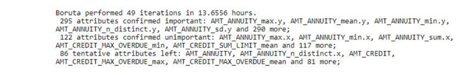
We then applied the the same data preprocessing steps to clean the fully joined dataset. This time, we chose
to remove columns with more than 50% missing values before applying mice for missing value imputation, this returned
a total of 593 variables in our full dataset. We then used Boruta to perform feature selection and returned 295 variables in the
dataset ready for modeling:
Final Result
We ran a total of three models on the full dataset: logistic regression, LightGBM and XGBoost. You may elect to run models on h2o or write codes to run each model separately. Below is how to build a XGBoost in code:
library(dplyr)
library(tidyr)
library(readr)
library(haven)
library(xgboost)
library(caret)
#import final dataset previously saved
df <- read.csv(file="cleaned_fulltable.csv")
#create index column tri
tri <- 1:nrow(df)
y <- df$TARGET
df <- df %>%
select(-TARGET, -SK_ID_CURR)
df <- df %>%
data.matrix()
#split data into train and test sets
library(magrittr)
tr_te <- df[tri, ]
tri <- caret::createDataPartition(y, p = 0.8, list = F) %>% c()
dtrain <- xgb.DMatrix(data = df[tri, ], label = y[tri])
dval <- xgb.DMatrix(data = df[-tri, ], label = y[-tri])
cols <- colnames(df)
#rm(tr_te, y, tri); gc()
#set parameters in XGBoost model - tune in accordance to result
p <- list(objective = "binary:logistic",
booster = "gbtree",
eval_metric = "auc",
nthread = 4,
eta = 0.05,
max_depth = 6,
min_child_weight = 30,
gamma = 0,
subsample = 0.85,
colsample_bytree = 0.7,
colsample_bylevel = 0.632,
alpha = 0,
lambda = 0,
nrounds = 2000)
set.seed(0)
m_xgb <- xgb.train(p, dtrain, p$nrounds, list(val = dval), print_every_n = 50, early_stopping_rounds = 600)
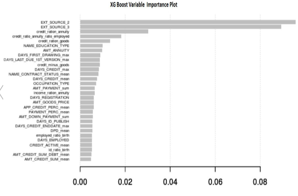
#create importance plot
xgb.importance(cols, model=m_xgb) %>%
xgb.plot.importance(top_n = 30)
Below is a chart comparing accuracy results from each model:
| Model | Training Data AUC | Testing Data AUC |
|---|---|---|
| Logistic Regression | 70.35% | 70.7% |
| XG Boost | 78.04% | 77.49% |
| Light GBM | 80.80% | 78.38% |
Our two final best models are LightGBM and XGBoost.
LIghtGBM –Result: This method performed best with significant regularization on test data
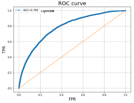
XG – Boost Result: Our XG-boost model gave 77.6 % AUC, which is the second-best AUC performance we have thus far.
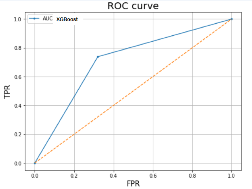
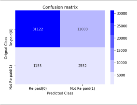
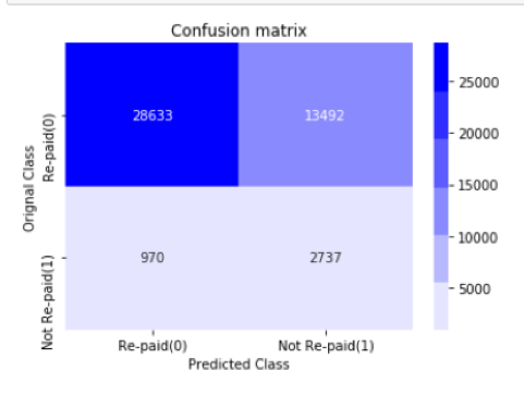
If using AUC as the primary performance metric, our LightGBM model (78%) has superior performance compared to XGboost (77%). However, we also used confusion matrix as a secondary performance metric. As shown below, the number of true negatives has increased in results given by the xgboost model. According to this confusion matrix, our precision on target class 1 is 74%. As previously explained, we wanted to minimize the number of false negatives as much as possible so that we can accurately predict default loans. As a result, we concluded that both models are on par in terms of performance using a combination of confusion matrix and AUC metrics.
Variable Importance Plot:
References
Thank you for the patience if you read till the end. 💛 I'm always looking for new opportunities to improve and please feel free to connect on LinkedIn if you're interested in data science like me.


Facebook
LinkedIn
Email